Our goal was running real-time instance segmentation on the Hailo-10H while preserving its open-vocabulary capability. This article covers the full path from model to a end-to-end pipeline: the model adaptation that makes runtime prompting possible, compilation to the Hailo accelerator at two resolutions (640×640 and 320×320), the Python pipeline from camera acquisition to display, the optimization journey that took the demo from 6.3 FPS to 15.6 FPS (640px) and ~31 FPS (320px), and a head-to-head benchmark of the two resolutions on the same hardware.

Why “prompt anything” segmentation

We replace fixed-class networks and retraining cycles with a single edge deployment that segments any user text prompt. Instance segmentation on the edge usually means a fixed, closed set of classes baked into the model at training time. If you want to segment something the model was not trained on, you retrain and re-export your model. That is costly and time-consuming.

YOLOE-26 breaks that assumption: it is an open-vocabulary (“prompt anything”) segmentation model. You give it text prompts at runtime, e.g., person, forklift, solar panel, red flower,  and it segments those classes with no retraining and no model rebuild. For warehouse/AMR object handling, agricultural and inspection use cases, and rapid prototyping where the class list changes faster than a training pipeline can keep up. The new wave of Discrete NPU (DNPU) unlock this type of heavier processing that gave more flexible capability to computer vision application. We leverage a Hailo-10H on a Raspberry Pi AI HAT+ 2, combined with a Raspbery Pi 5.

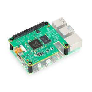
Hailo-10H on a Raspberry Pi AI HAT+ 2

The model: prompt-invariant open vocabulary

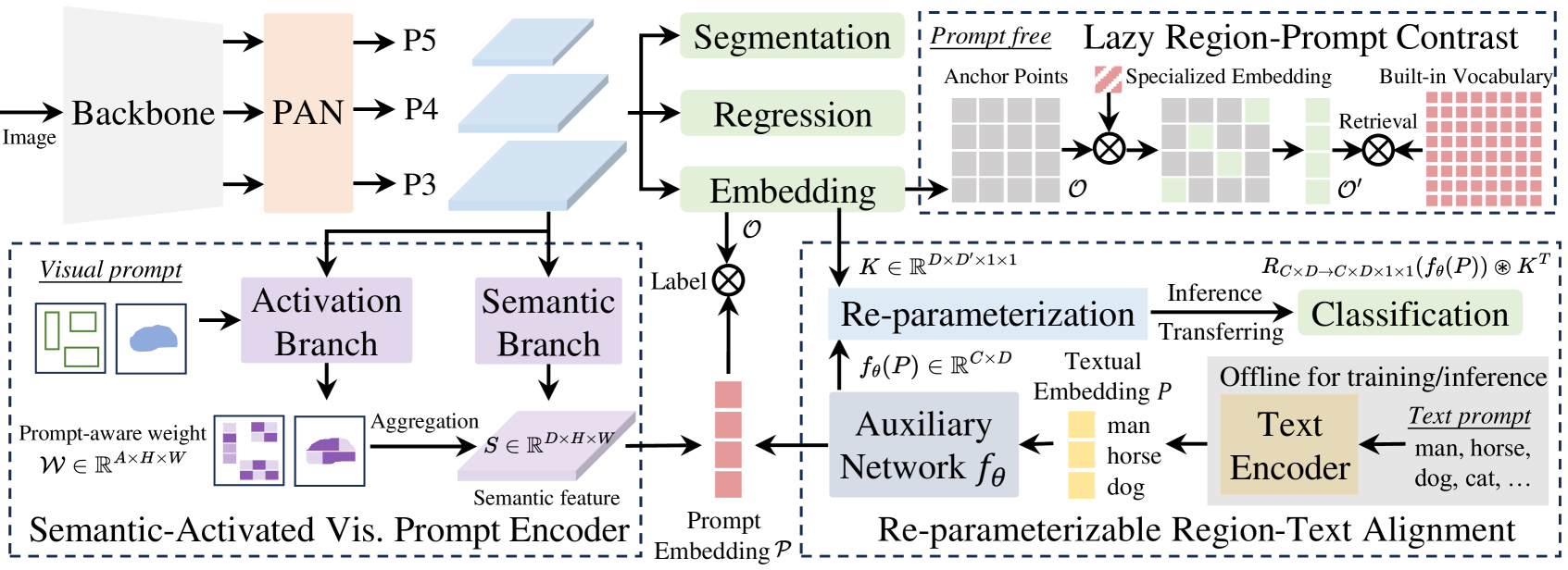
YOLOE (Real-Time Seeing Anything) is a new advancement in zero-shot, promptable YOLO models, designed for open-vocabulary detection and segmentation. Unlike previous YOLO models limited to fixed categories, YOLOE uses text, image, or internal vocabulary prompts, enabling real-time detection of any object class.

https://docs.ultralytics.com/models/yoloe

YOLOE’s segmentation head is contrastive: it scores each spatial location against a set of text embeddings. Class scores are dot products of backbone image embeddings and text embeddings, scaled and biased per level:

score = image_embedding · text_embedding × exp(logit_scale) + bias

YOLOE : Real-Time Seeing Anything – https://arxiv.org/html/2503.07465v1

This structure is the key to running open-vocabulary inference on a fixed accelerator. The image embeddings do not depend on the prompt. So we split the model:

• NPU (fixed graph): the backbone generates image embeddings, raw boxes, mask coefficients, and prototypes per frame.
• On the CPU (runtime): the active prompt list is scored against those image embeddings, then decoded into boxes and instance masks.

With this prompt-invariant split, changing prompts, even to a class the demo has never seen, costs only a CPU re-score. No HEF recompile, no camera restart. The split is mathematically exact: the contrastive head’s scoring decomposes cleanly into an NPU part (image embeddings) and a CPU part (dot product, scale, bias), verified against the reference model with a max score difference of 6×10⁻⁴ across 3, 10 and 80 active prompts.

True free-text prompting: the on-device text encoder

The prompt-invariant split answers where prompt scoring happens, but it leaves a question open: where do the text embeddings come from? A precomputed cache (e.g. the 80 COCO class names) is enough for a fixed demo — but it quietly reintroduces the closed vocabulary we set out to eliminate. YOLOE-26s-seg was trained on 1200+ classes; limiting it to a cache wastes the model. The ultimate version of this pipeline encodes arbitrary text on the device itself, at runtime.

On-Device Text Encoder Architecture

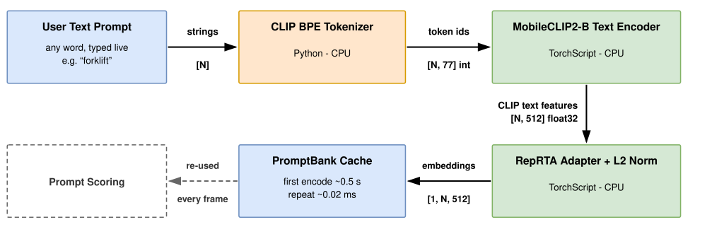
For true free-text prompting (beyond a precomputed class cache), we deployed an on-device MobileCLIP2-B + RepRTA text encoder, so the operator can type any word and have it encoded and segmented live.

To do that, the demo embeds the full YOLOE text path on-device, describe as follows:

On-Device Text Encoder Architecture

• Tokenizer: a vendored, pure-Python CLIP BPE tokenizer — no ultralytics, open_clip, clip or onnxruntime on the Pi.
• Text encoder: MobileCLIP2-B as a TorchScript module (mobileclip2_b.ts, 243 MB, pinned and SHA256-checked Ultralytics release asset), running on the Pi CPU via torch.
• RepRTA adapter: YOLOE’s text-side adapter, exported to TorchScript (reprta.ts), followed by L2 normalization.

Verified end to end on the device, in the same process as HailoRT, against workstation references over a word set including out-of-COCO terms: max abs diff 5.59×10⁻⁷. Whatever the operator types, the edge device computes the same prompt embedding the full PyTorch model would.

At runtime, any prompt not already in the bank is encoded on the spot, appended, and cached. The first encode of a new word costs ~0.5 s on the device CPU (plus a one-time ~2 s TorchScript warmup at first use); repeats hit the cache in ~0.02 ms. This runs off the hot loop, preserving frame pipeline speed while encoding new words in the background.

The complete demo therefore runs three cooperating compute stages: the text encoder on the CPU (on demand, cached), the vision backbone on the NPU (every frame, fixed), and the contrastive scoring + decode on the CPU (every frame, prompt-dependent).

Model adaptation for the NPU: the raw-head cut

The Hailo parser rejects post-processing tail operations like TopK, GatherElements, and dynamic Gathers on NPU.

The fix is a raw-head cut: the ONNX graph is cut before the decode/NMS tail, exposing the raw backbone heads as outputs. Everything past the cut (scoring, DFL box decode, top-k, mask assembly) moves to the CPU, which is exactly where the prompt-invariant split wants it anyway. The accelerator runs only the part that is both prompt-independent and NPU-friendly.

A second, subtler issue: the raw graph still failed the parser with ValueError: channels is not in list on the attention Split nodes (dynamic Shape/Slice/Gather). Running onnxsim with fixed input shapes (images=[1,3,H,W]) resolves dynamic shapes for compilation. Static input shapes are mandatory for both the ONNX export and the Hailo compile.

Quantization: INT8 via the Hailo Dataflow Compiler (level 4)

The NPU runs INT8. We compile using Hailo Dataflow Compiler Level 4 optimization with 1,024 validation calibration images. Normalization (/255) is baked into the graph via the model script (.alls), so the HEF accepts uint8 NHWC directly and there is no CPU-side float conversion in the hot loop.

Two compile properties matter:

1. Multi-context is required. A single-context compile fails with Resources presolve failed: lcus=(…/80); the compiler partitions the network into 6–7 contexts and succeeds.
2. Calibration normalization must match inference normalization exactly. A mismatch here silently produces garbage masks. The calibration tensors are letterboxed and uint8-encoded the same way the runtime preprocesses each frame.

The pipeline: camera to display

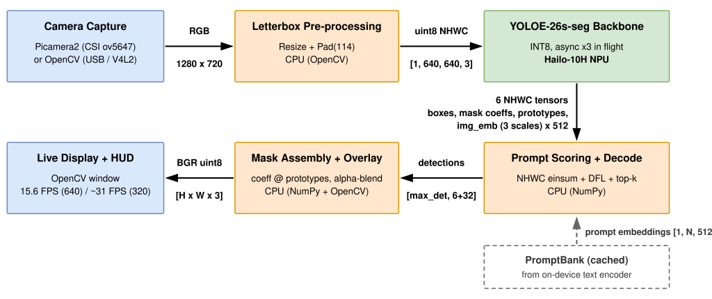
Our pure-Python pipeline uses Picamera2/OpenCV for capture, HailoRT APIs for inference, and OpenCV for rendering.

The pipeline architecture is:

Pipeline Architecture

The accelerator emits six NHWC tensors (boxes, mask coefficients, prototypes, and three image-embedding scales). The CPU scores the active prompts against the embeddings, decodes only the surviving detections, builds one instance mask per detection, and alpha-blends them into the display frame. The prompt path (text → embedding) is cached off the hot loop, so steady-state cost is dominated by the NPU and the number of active prompts.

Crucially, the loop is not run serially. A naive serial loop pays capture + inference + post per frame. The shipped pipeline runs Hailo inference on a worker thread with async double-buffering (3 inferences in flight), so a finished frame emerges every NPU-bound period instead of every round trip. This is the single biggest throughput lever, see details below.

Optimization journey

The first working demo ran at ~5.5 FPS (640px), strictly serial, NPU and CPU never overlapping. The headline steps:

Two findings drove everything:

1. The biggest CPU cost was not real computation. Almost half the per-frame CPU time was spent transposing the six HEF outputs from the accelerator’s native NHWC layout to BCHW, ~22 MB of memory copies per frame (~58 ms). Rewriting the consumers (scoring, box decode, mask assembly) to read NHWC directly, e.g. changing the scoring einsum from bchw,bkc->bkhw to bhwc,bkc->bkhw, is mathematically identical and dropped the map step from ~58 ms to effectively zero. Key Takeway: match the accelerator’s native tensor layout instead of fighting it.
2. Latency and throughput are different numbers. A single NPU inference is a ~110 ms round trip (640px), but the Hailo-10H is internally pipelined and holds up to ~10 frames in flight. Fed continuously via async double-buffering, a finished frame emerges every ~64 ms -> the NPU compute stage, even though each individual frame still takes ~110 ms end to end. The ~110 ms round trip decomposes into ~64 ms of NPU compute (the bottleneck) plus ~48 ms of overlappable DMA + driver/scheduler time.

After these optimizations the demo is throughput-bound at the ~64 ms NPU stage (640px).

Results and performance

We benchmarked two compiled models at 640px and 320 px resolution with the same configuration:

640px vs 320px (synchronous per-image harness)

Live demo throughput (async double-buffered pipeline, depth-3)

Takeaways:

• Resolution is the dominant speed lever. Halving the input (640→320) gives ~3.6× faster NPU inference. The full-pipeline gain is slightly smaller (~3.1×) because the fixed CPU-side cost (scoring, decode, mask reconstruction) does not shrink proportionally.
• The cost is small-object mask precision. 320px loses ~0.095 mask IoU, almost entirely recall on small objects that the coarser 320 grid (2100 anchors, 80×80 proto) resolves less finely than 640 (8400 anchors, 160×160 proto). The 320px ONNX float reference already drops to 0.672 before quantization, this is the model’s inherent resolution trade-off, not a quantization artifact.
• Active prompt count is the second speed lever. NPU inference is constant per resolution; CPU prompt scoring grows ~1.5 ms per active prompt, and CPU mask assembly grows with the detection count. Empty/few prompts → NPU-bound (~31 FPS at 320). 80 prompts → CPU-bound (~12 FPS at 320). Keep the active prompt set small for the smoothest frame rate.

Use 320px when throughput/latency/power matter more than fine mask precision. Use 640px when mask quality on small objects is the priority.

Key engineering takeaways

Deploying an open-vocabulary segmentation model on an NPU is not plug-and-play. Several lessons emerged from this project:

1. Split the model along the prompt-invariance boundary. Splitting the backbone (NPU) from prompt scoring (CPU) enables open-vocabulary inference on fixed accelerators. Any prompt, no recompile.
2. Match the accelerator’s native tensor layout. The biggest single CPU win came not from smarter math but from deleting per-frame NHWC→BCHW transposes and reading the NPU’s native layout directly. ~58 ms → ~0 ms.
3. Latency ≠ throughput on a pipelined NPU. Async double-buffering turned a 110 ms-latency inference into a 64 ms-throughput stage by overlapping DMA/driver time across frames. Measure the period between completions, not the per-frame round trip.
4. Calibration must mirror inference exactly. Identical letterbox + uint8 + normalization in calibration and runtime; baking normalization into the compiled model removes a whole class of preprocessing bugs and a per-frame float conversion.
5. Resolution is a first-class deployment knob. Two compiled version from one model give a clean throughput/quality dial (3.6× speed for ~0.095 IoU) selectable at launch. No retrain.

Conclusion

We demonstrated real-time, open-vocabulary segmentation on Hailo-10H using YOLOE-26s-seg with an edge-optimized model split. The operator types a class, the NPU segments it, with no model rebuild. The path from a PyTorch model to a fluid live demo required deliberate engineering at every layer: a raw-head graph cut for NPU operator compatibility, INT8 L4 quantization with calibration that mirrors inference, a layout-aware Python pipeline from camera to display, and async double-buffering that exploits the NPU’s internal pipelining to reach the device’s true throughput ceiling.

Open-vocabulary segmentation on low-power hardware applies wherever the class list changes faster than a retraining cycle: warehouse and AMR object handling, agricultural inspection, industrial defect triage, and rapid prototyping. The value proposition is to replace a fixed-class network and its retraining loop with a single edge deployment driven by plain text.

The result is a complete, reproducible edge stack that turns a single camera feed into a live, promptable instance-segmentation view, at ~15.6 FPS (640px) or ~31 FPS (320px),on a power-efficient platform, with resolution and prompt set as runtime dials.