Optimizing Instance Segmentation application on Renesas RZ/V2H

Running instance segmentation in real time on embedded hardware takes more than just a fast model. Camera capture, image preparation, inference, mask creation, drawing, and display, all of which have to fit in the time budget of a single frame. This article covers how we optimized that whole path on the Renesas RZ/V2H.

We started by timing every stage from the USB camera to the screen. Model inference is a key part of the pipeline, but in this application it was not the biggest bottleneck. CPU image processing and display work took more time. We optimized the pipeline as a whole, starting with the largest sources of delay. The result was significant: the frame rate rose from about 11 to roughly 27 to 29 frames per second.

With those larger bottlenecks out of the way, we then evaluated model pruning as the next part of the optimization process. Pruning sets less useful weights to zero so that supported hardware can skip some of the work. We tested pruning instance segmentation models from three YOLO families to see how it affected inference time and deployment size on DRP-AI3.

In an earlier YOLO project, we used text prompts to select what the model should segment. You can read about that project here.

The full program, not only the model

All tests ran on a Renesas RZ/V2H board. Four Arm Cortex-A55 CPU cores run the program and the image work, a dedicated accelerator called DRP-AI3 runs the neural network, and a Mali-G31 graphics processor helps draw the final image.

Runtime setup

The four CPU cores ran at 1.2 GHz and DRP-AI3 at 1 GHz. The camera supplied images, and the segmentation models took a fixed 224 × 224 input. Every test used the same board settings, camera size, and full-screen display path.

When we compared the old and new versions of the program, both used the same YOLOv8n segmentation model, so any change in frame rate came from the code around it. The pruning test later did the opposite: it kept the improved program fixed and changed only the deployed model.

Throughout this article, inference means running the neural network on DRP-AI3. That is only one stage. The rest covers camera capture, model input, mask creation, drawing, and display.

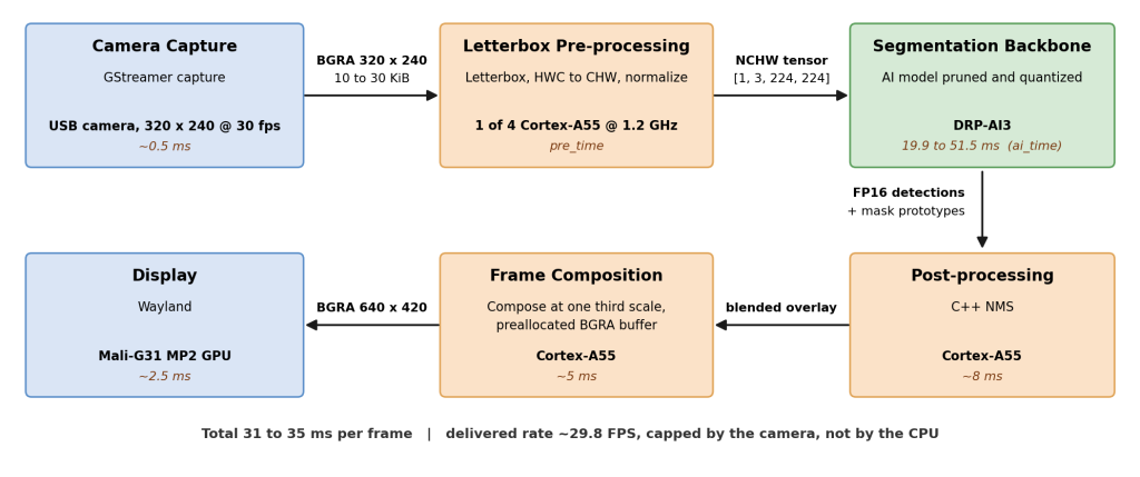
The basic flow stayed the same in both versions. The Linux V4L2 camera interface receives a frame, and GStreamer converts it into a BGR image, which stores blue, green, and red values for each pixel. The CPU then resizes that image to 224 × 224, padding it where needed to keep the proportions.

The CPU rearranges the pixels into the channel-first layout the model expects and normalizes the values. DRP-AI3 then runs the network, which returns object boxes, confidence scores, and the data needed to build masks.

After inference, the CPU removes duplicate boxes for the same object, builds the masks, draws everything, and assembles the display image. The display stack hands that image to the graphics processor, which scales it, and Weston puts it on screen.

The camera-to-display flow

Why we started outside the model

At first, the model seemed like the obvious thing to work on. Then we measured the frame times. The first version of the program needed roughly 90 to 130 ms (milliseconds) per frame, which is about 8 to 11 frames per second, and the model accounted for only 25 to 30 ms of that. Most of the delay was somewhere else.

We started by measuring the complete frame

We split each frame into broad stages and timed each one. The numbers below come from a single test run, so treat them as rough. They were enough to tell us where to work first.

The timers covered camera capture, model input, DRP-AI3 inference, output work, frame building, and display. Since camera capture includes time spent waiting for the next frame, we tracked both the processing time and the wall-clock gap between displayed frames. That gap is what gives the real delivered frame rate.

No single stage was responsible for the whole delay, but several of them repeated work on large images. The program enlarged the camera image too early, then copied, converted, blended, and uploaded that large image several times. Some steps also ran once per detected object.

Our plan followed from that: shrink the images the CPU handles, remove the repeated mask and drawing work, and cut down the camera input data. The model stayed untouched.

Optimizing the non-inference stages

Build a smaller frame and scale it for display

The largest gain came from separating the processing size from the display size. Originally, the CPU built the whole image at full display size (1920×1080). Now it builds a 640 × 420 image and lets the graphics processor scale it up to the full-screen window.

The full window is 1920 × 1260 including the title area. The old version enlarged the camera result to 1440 × 1080 before placing it in that window. The new one enlarges it only to 480 × 360 and composes the full frame at 640 × 420. The window itself stays the same size.

Each full-image step now handles roughly 1.1 MiB instead of 9.7 MiB, and the final enlargement lands on the graphics processor, which is built for exactly that job. In our test this change alone saved roughly 25 to 30 ms per frame.

Generate all masks together

An instance-segmentation model produces a separate mask for each object. For every detection it returns 32 mask coefficients, along with one mask prototype shared by all detections. The old program multiplied each set of coefficients by the prototype separately, so every object triggered a new matrix operation and another read of the same prototype.

The new program stacks the coefficients for all detections into one matrix, and a single larger multiplication produces every mask at once. We also cap each frame at eight displayed masks so that crowded scenes cannot cause long delays. Together these changes saved roughly 10 to 15 ms.

Blend once per frame

The original drawing path created and blended a full-image overlay for every object, so eight objects meant eight copies and eight blends. The revised path draws all objects on a single overlay and blends it once.

Each mask still decides which pixels get the object’s colour. The difference is that the program waits until every mask is on the shared overlay before combining it with the camera image. The visible result is identical, and depending on the number of objects this saved roughly 8 to 20 ms per frame.

Convert the small image, not the large one

The camera path provides a three-channel BGR image, while the display path uses BGRA, which adds an alpha channel for blending. The program used to run this conversion on the large display image. We moved it to the small 320 × 240 camera image instead and kept BGRA through the rest of the composition.

Fixed items such as the title area are now prepared once and reused, and display buffers are reused instead of recreated every frame. The result is the same image with less work.

Use compressed camera input

The original camera path transferred raw YUYV frames. The new one asks the camera for MJPEG, a compressed format it supports. At 320 × 240, an MJPEG frame was roughly 10 to 30 KiB against about 150 KiB for raw YUYV.

GStreamer decodes the JPEG frame and converts it to the BGR format the program uses. Decoding added less than a millisecond in our run, and far less data travels over USB. It was a minor gain overall. Most of the improvement still came from the smaller display images.

Result of the program changes

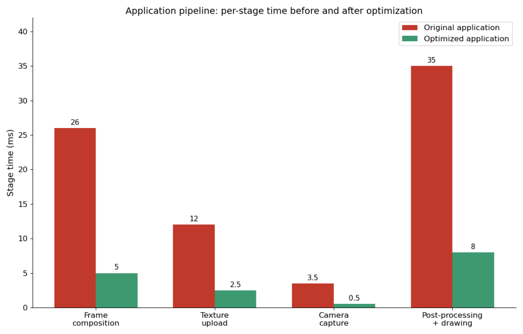
The model stayed the same for this comparison, so the numbers below show only the effect of the program changes. The values are rounded and come from one run.

In most runs the frame rate rose from about 11 to roughly 27 to 29 frames per second, close to the camera’s 30-frame limit. None of this touched the model. We simply removed repeated work and moved image scaling to the graphics processor.

After these changes, inference took up a larger share of each frame, which meant model changes could finally make a visible difference. So we returned to pruning.

Returning to pruning instance segmentation models

A neural network contains millions of learned values called weights. Pruning sets the less useful ones to zero during or after training, with the goal of reducing work without losing too much accuracy.

Weight pruning and channel pruning

There are two broad ways to prune a model. Weight pruning zeroes individual weights but leaves every layer at its original size. Channel pruning removes whole groups of values, which changes layer sizes and the model graph. It can remove more work, but it also cuts deeper into the network and usually needs more retraining.

We used the weight-pruning method from the Renesas DRP-AI Extension Pack, so the exported model keeps the same layer shapes as the unpruned one, and its ONNX file stays about the same size. The compiled file for DRP-AI3 can still shrink, because the compiler stores the zeroed weights in a compact form.

How DRP-AI3 uses sparse weights

DRP-AI3 uses a flexible N:M pruning pattern. The tools divide the weights into small groups of M candidates and keep the N most useful values in each group, and N can vary between groups. That gives the hardware a regular layout while letting each part of the model keep a different number of weights.

A model with 70% of its weights pruned will not simply run 70% faster, though. Unpruned parts still run, data still moves between steps, and the output still needs processing. The actual gain depends on the model and on which work DRP-AI3 can skip.

Before deployment, every model is also converted to a compact 8-bit integer format, a step called quantization. We used the same calibration images, quantizer settings, and compiler settings for the unpruned and pruned versions, so pruning rate and model family were the only planned differences in the test.

For the pruning instance segmentation test we used three large YOLO models: YOLOv8l, YOLO11l, and YOLO26l, each in an unpruned baseline plus 70% and 90% pruned versions. All of them used a 224 × 224 input and the same improved program. Each result is the average of one 200-frame run after a warm-up frame, so this is one controlled test rather than a broad study.

The program resized each 320 × 240 camera frame down to the 224 × 224 model input, with padding. The full-screen display stayed active during the runs, so the measurements come from the deployed camera application rather than a model-only benchmark tool.

Pruning results on the target board

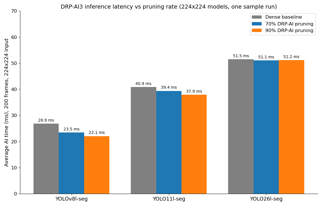
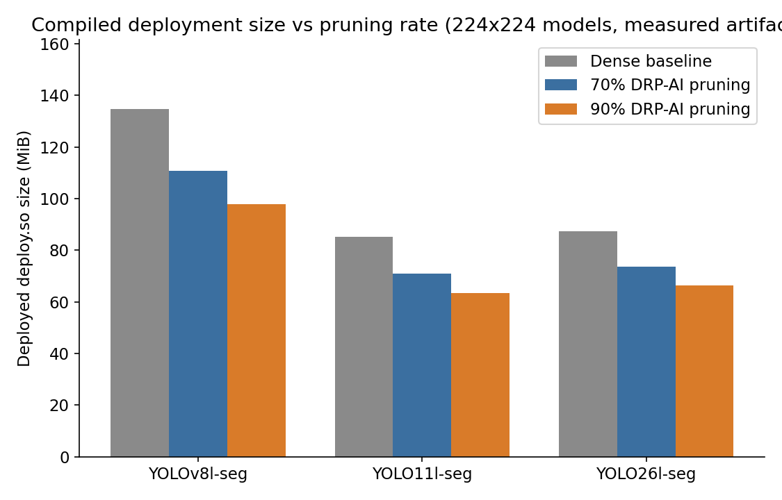
Here we timed only the model running on DRP-AI3. Camera capture, model input, masks, drawing, and display are excluded. We also recorded the compiled model size. As before, the values are rounded because they come from one run.

YOLOv8l benefited the most

YOLOv8l showed the clearest gain. Inference fell from roughly 27 ms to 24 ms at 70% pruning and to 22 ms at 90%, about 13% and 18% faster. The compiled model also shrank by about 18% and 27%.

Those gains are useful, but they sit far below the pruning rates. The number of zeroed weights clearly does not translate directly into speed.

YOLO11l improved modestly

YOLO11l fell from roughly 41 ms to 38 ms at 90% pruning, about 7% faster, and its compiled model was about a quarter smaller. Pruning helped both speed and storage here, but the speed gain was modest.

YOLO26l became smaller, but not faster

YOLO26l stayed near 51 ms across all three versions, even though its 90% pruned model was about 24% smaller. A smaller model file clearly does not guarantee faster inference.

The likely reason lies in the exported graph. YOLOv8 and YOLO11 return raw detections and leave it to the CPU to remove duplicate boxes afterwards, a step commonly called non-maximum suppression. YOLO26 does that work inside the deployed model.

Its graph has to reshape, reorder, join, and select output data. None of those steps contain convolution weights, so weight pruning cannot shrink them, and their cost stays the same even when the compiled file gets smaller. Data movement and scheduling add fixed time on top.

The same pruning rate can therefore play out very differently across models. The only reliable check is to run the compiled model on the target board. Weight counts and file sizes are no substitute for timing it.

A note about model accuracy

Speed is only half of the decision. Pruning removes learned information, so the model has to be retrained and its accuracy checked. Our retraining runs were short because this test focused on timing.

Each model trained for ten epochs on about 3% of the COCO training set, roughly 3,500 images, with a batch size of 64 and the same short schedule for every variant. Validation ran once at the end. That kept the variants comparable, but it was nowhere near long enough for training to settle.

The most heavily pruned models did lose segmentation accuracy, so treat these as timing results, not deployment targets. A production model needs longer training, tests on data from its real use case, and possibly a lower pruning rate if the accuracy loss stays too high.

The test still answers its main question, which is how pruning changes DRP-AI3 inference time. Picking a final model would also require a proper accuracy study.

What we learned

1. Measure the full frame first. Inference took about one quarter of the old frame time. Starting with the model would have missed the larger costs.
2. Remove repeated image work. Smaller images, combined mask processing, and one blend per frame produced the largest gains.
3. Give each hardware block suitable work. The CPU handles the program, DRP-AI3 runs the model, and the graphics processor scales the display image.
4. Pruning rate does not predict speed. When pruning instance segmentation models at 90%, the gain ranged from about 18% for YOLOv8l to almost zero for YOLO26l.
5. Smaller does not always mean faster. All three models used less storage after pruning, but only two ran faster.
6. Accuracy still matters. Heavy pruning may save time or storage, but it can require more training to recover useful results.

Conclusion

The first version of the program ran at roughly 8 to 11 frames per second, and most of its delay sat outside DRP-AI3. That is why we started with the rest of the program instead of the model.

Using a smaller display image produced the largest gain, and combined mask work, a single blend, smaller image conversion, reused buffers, and compressed camera input removed more on top. With the same model, the program usually reached roughly 27 to 29 frames per second, close to the camera’s limit of 30.

Then we tested pruning instance segmentation models. At 90% pruning, YOLOv8l ran about 18% faster, YOLO11l about 7% faster, and YOLO26l became smaller without running faster. Each model reacted differently.

Neither program work nor model work is always more important. It depends on where the frames actually spend their time. Here, work outside inference was the first limit, so we addressed it first. After that, pruning could reduce part of the remaining time.

Optimizing embedded AI is a whole-system job. Measure the path from camera to display, give each processor the work it is good at, and test the model on the target board with an eye on accuracy. Had we looked only at the neural network, we would have missed most of the gain in this project.

References

• Renesas, Next Generation Highly Power-Efficient AI Accelerator DRP-AI3, February 2024
• RZ/V2H DRP-AI TVM: https://github.com/renesas-rz/rzv_drp-ai_tvm
• DRP-AI pruning examples: https://github.com/renesas-rz/rzv_drp-ai_tvm/tree/main/pruning
• DRP-AI sample applications: https://github.com/renesas-rz/rzv_ai_sdk
• Ultralytics YOLO documentation: https://docs.ultralytics.com/