 In a previous post I described how to manipulate data extracted from a Saleae logic analyzer with Python, to view the latency between two digital signals and deduce the temporal jitter of one of them. In conclusion, I expressed the assumption that the Saleae SDK could allow us to retrieve information about the signals in real time, rather than via an intermediary CSV file. But at the end, the best solution I found came from a more generic free software.
The Saleae SDK solution
Saleae provides developers with two solutions:
- An API (in beta at the moment) that only allows to control their visualization software from a socket;
- A SDK that allows expanding their software and write your own protocol analyzer plugins.
We could have looked at the SDK and written a parser exporting the latency between two defined signals on the fly, but this solution is dependent on the Saleae software and its evolutions, ensuring very low durability. In addition, Saleae’s visualization software is not intended to be used with different types of logic analyzers. We were looking for a more generic and permanent solution.
Sigrok: an open-source software suite for logic analyzers
It was during a discussion with my colleagues that Emeric Vigier pointed to me a software called sigrok. Aiming to provide a free and generic logic analyzer, sigrok is a software suite for extracting data collected by various types of analyzers and displaying them or analyzing them using protocol decoder plugins.
This suite consists of several sub-projects:
- libsigrok: a library written in C that standardizes access to different test and measurement devices.
- libsigrokdecode: a C library that provides an API for protocol decoding. The decoders are written in Python 3 and later.
- sigrok-cli: a command line interface to manipulate sigrok.
- PulseView: a Qt GUI to manipulate sigrok.
- Fx2lafw: sigrok also provides an open source implementation of the Cypress FX2 chip firmware, which is used — among others — by Saleae in all versions of its logic analyzers except the logic Pro 16. This firmware can program the embedded logic to function as a single logic analyzer hardware.
Sigrok usage example
An end-to-end example will be better than a thousand words. We will use PulseView to capture and visualize signals from a logic analyzer.
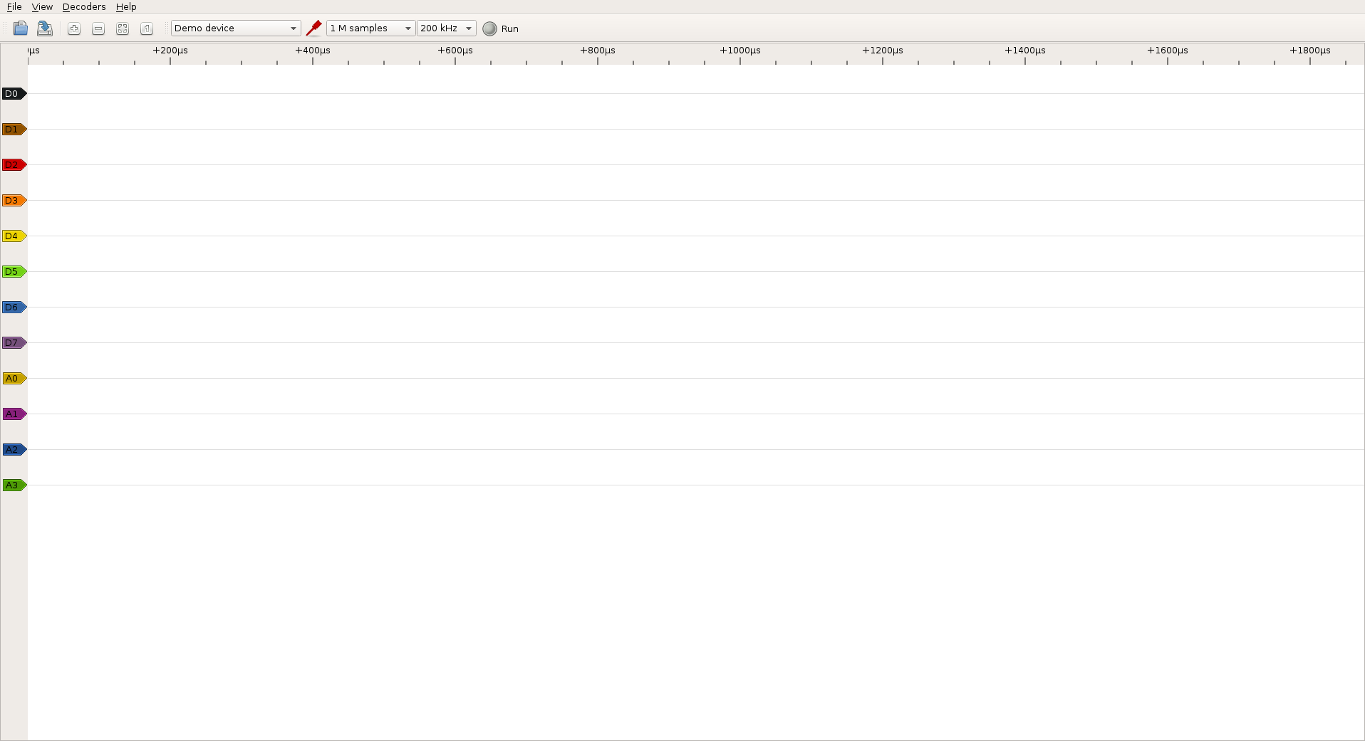
At startup, PulseView in its version 0.2.0 looks like this:
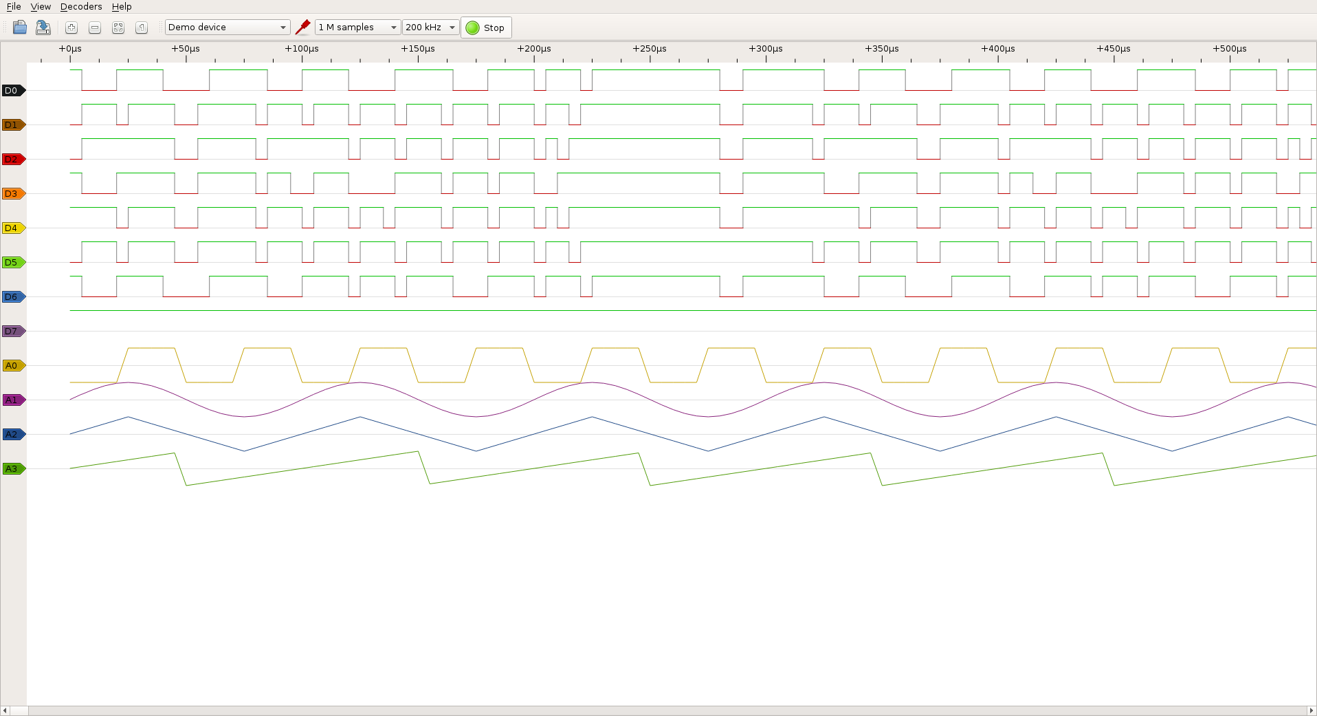
We’ll start a capture leaving the demonstration device generate random signals:
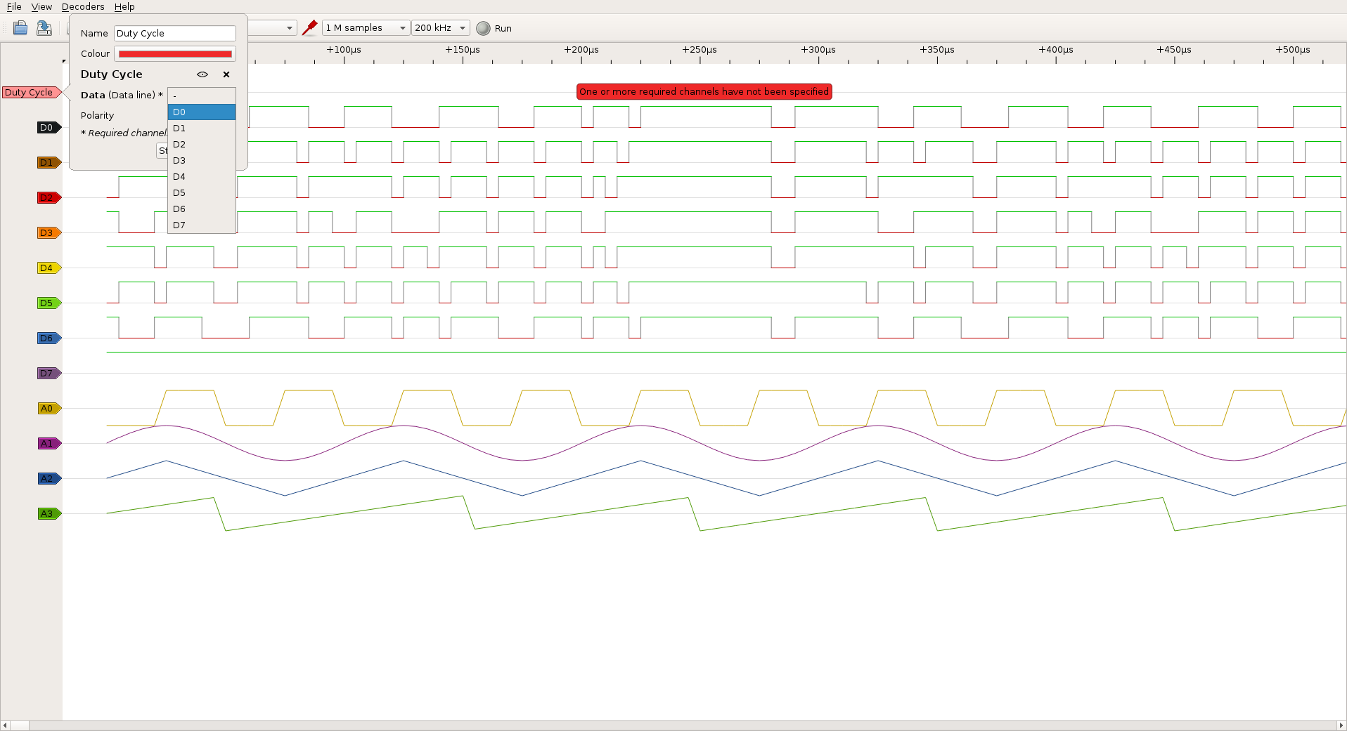
We will then add a pretty simple decoder that calculates the duty cycle of a digital signal:
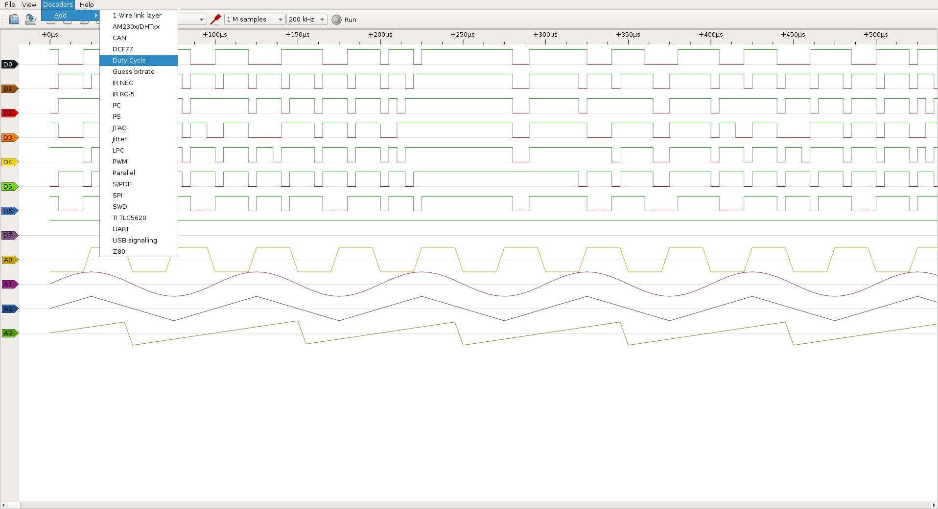
Each decoder has its options. In our case we simply set the channel on which we want to apply the decoder:
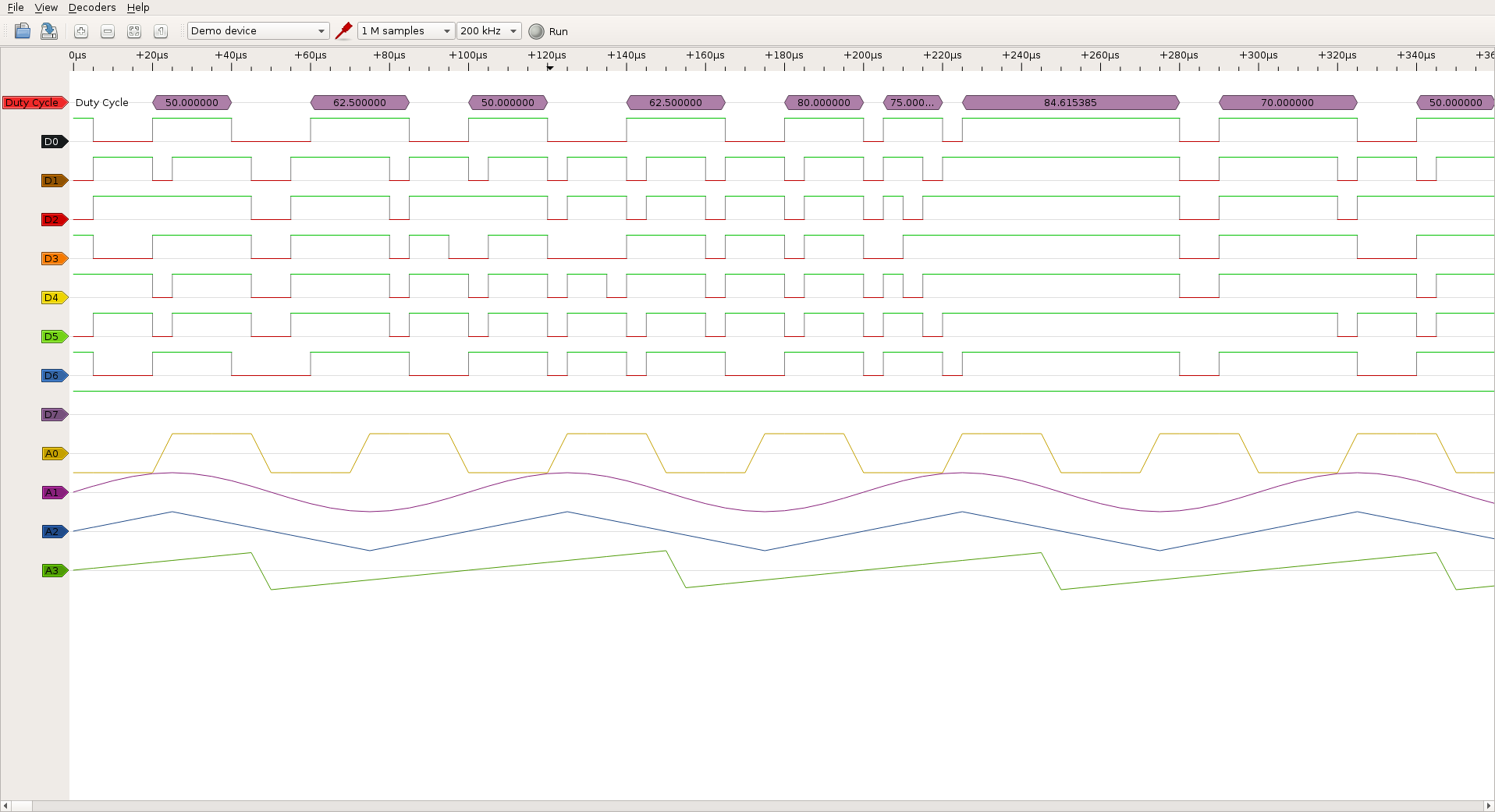
The duty cycle calculation is applied to the channel and displayed directly into PulseView:
Sigrok: writing a decoder for determining the latency between two digital signals
The following is based on the libsigrok and libsigrokdecode in their version 0.3.0.
Each protocol decoder is a Python module that has its own subdirectory in the libsigrokdecode decoders directory.
A decoder consists of two files:
- __ init __ py . This file is required to initialize the decoder and contains a simple description of the protocol
- pd.py : This file contains metadata about the decoder, and its implementation.
We’ll look at the file pd.py that contains the code for our decoder. The libsigrokdecode API provides all the information on the captured signals.
To calculate the latency between two digital signals, our logic is to consider one signal as a reference clock, and the other as a result of it. The two signals are linked so each state transition of the clock signal will result in the other signal to change also transition with a more or less variable latency. We will discuss the fluctuation of this latency later.
The decoder options
The first thing to do is to allow our channel decoder to define which signal corresponds to the reference clock, and which channel corresponds to the resulting signal. The decoder class precisely allows to define some attributes specifying its options, including one that allows the user to select channels:
class Decoder(srd.Decoder):
   # ...
   channels = (
      {'id': 'clk', 'name': 'Clock', 'desc': 'Clock reference channel'},
      {'id': 'sig', 'name': 'Resulting signal', 'desc': 'Resulting signal controlled by the clock'},
   )
   ...
The decode() method
The second step will consist in implementing the contents of the decode(). This method is called by the libsigrokdecode every time a new block of data is available for being processed.
Each block actually depends on the sampling rate of our signal. For example, sampling at 100Hz value, we get 100 blocks of data per second. The data blocks contain the sequence number of the current sample, as well as the status of various signals at this time.
From these informations, it is very easy to implement a state machine that will note how the sample transition occurred between the clock signal and the resulting signal. The number of samples elapsed between the two events multiplied by the sampling rate, gives us the latency in seconds.
In its simplified version, our state machine looks like this:
def decode(self, ss, es, data):

    self.oldpin, (clk, sig) = pins, pins

    # State machine:
    # For each sample we can move 2 steps forward in the state machine.
    while True:
        # Clock state has the lead.
        if self.state == 'CLK':
            if self.clk_start == self.samplenum:
                # Clock transition already treated.
                # We have done everything we can with this sample.
                break
            else:
                if self.clk_edge(self.oldclk, clk) is True:
                    # Clock edge found.
                    # We note the sample and move to the next state.
                    self.clk_start = self.samplenum
                    self.state = 'SIG'

        if self.state == 'SIG':
            if self.sig_start == self.samplenum:
                # Signal transition already treated.
                # We have done everything we can with this sample.
                break
            else:
                if self.sig_edge(self.oldsig, sig) is True:
                    # Signal edge found.
                    # We note the sample, calculate the latency
                    # and move to the next state.
                    self.sig_start = self.samplenum
                    self.state = 'CLK'
                    # Calculate and report the latency.
                    self.putx((self.sig_start - self.clk_start) / self.samplerate)

    # Save current CLK/SIG values for the next round.
    self.oldclk, self.oldsig = clk, sig
The outputs of our decoder
The libsigrokdecode library offers different ways of feeding information back to our decoder. A register() method allows to record the output data our decoder generates. Each output has a defined type; for example, type OUTPUT_ANN is used to define an annotation type output that will be represented in PulseView by graphic widgets that we saw previously in the duty cycle decoder example.
In our example decoder, we mainly use two types of outputs:
- An annotation type output (OUTPUT_ANN) to visualize latency informations in PulseView
- A binary type output (OUTPUT_BINARY) to output raw latency values for later analysis.
The final version of our decoder also includes a metadata output (OUTPUT_META) reporting statistics on missed signals. But that’s not relevant here.
Both outputs are defined as follows in our decoder:
self.out_ann = self.register(srd.OUTPUT_ANN)
self.out_bin = self.register(srd.OUTPUT_BINARY)
To report information about these outputs we use the put () method, which has the prototype:
put(start_sample, end_sample, output_type, data)
where output_type is one of previously defined methods (out_ann, out_bin).
To report the latency between two signals using standard annotations, for example, let’s write:
put(clk_start, sig_start, out_ann, [0, [my_latency]])
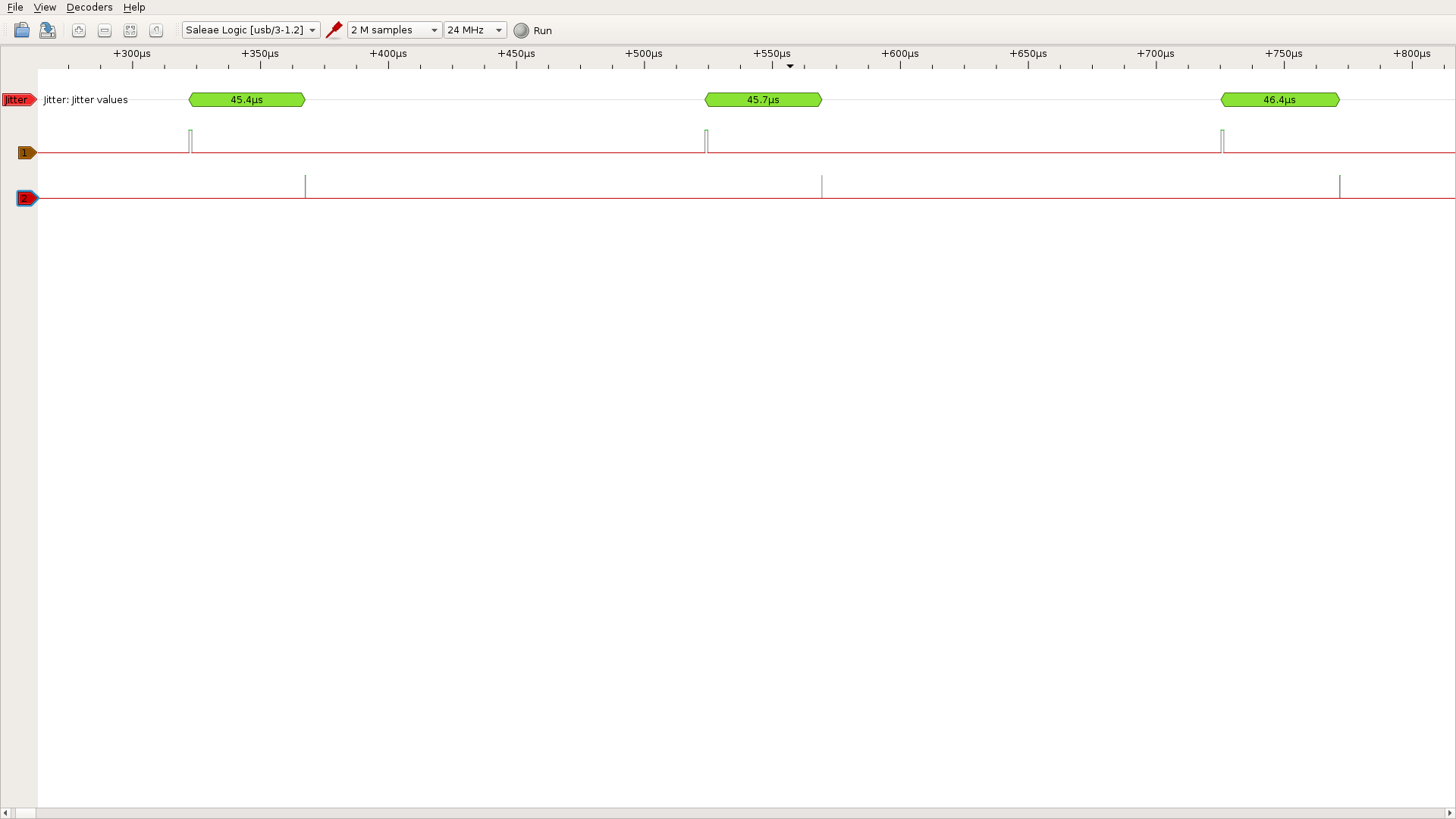
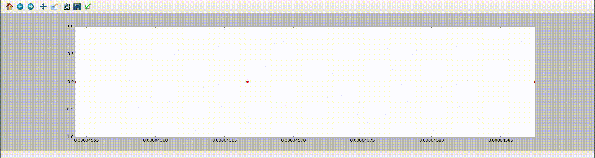
Results obtained with our latency decoder
Here is an example of the results obtained with our decoder in PulseView:
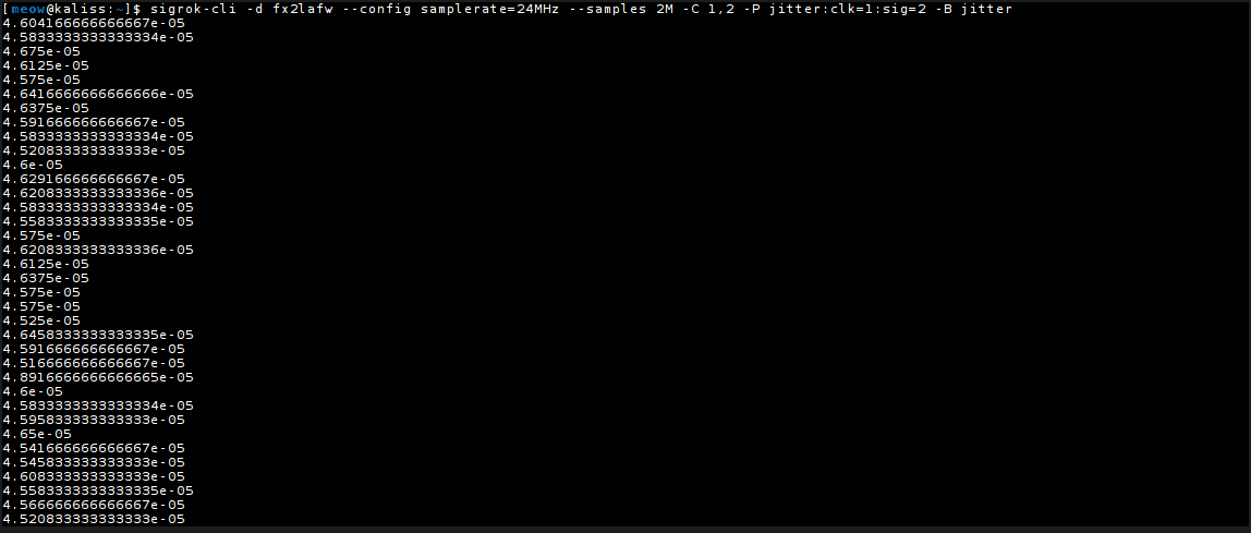
And the results obtained with sigrok-cli in its version 0.5.0 — including the binary output for raw latency values:
Viewing real-time data to determine the temporal jitter
As we have seen, sigrok-cli allows us to get the raw latency values on the console in real time. We will now turn our attention to variations of this latency. Indeed, there is no guarantee that the latency between these two signals is constant over the time.
Considering that the clock signal is periodic and without fluctuation, in theory, the resulting signal should be good and the latency between these two signals should be constant. If this is not the case, it is because there is a fluctuation of latency that we have described in the previous section as the temporal jitter of a signal, and this is what we see now.
We can imagine retrieving those values on the fly and displaying them in a graph. To do this, we would once again write a Python script.
I had a look at the matplotlib library and its animation module which provides a FuncAnimation() feature, to define a function that we’ll call in order to update the chart whenever new data is available. This function takes parameters such as the figure we are working on, the animation function to call, and the data set to be processed.
anim = animation.FuncAnimation(fig, animate, frames=data_gen)
These data can be in the form of a Python generator that will pair well with the reading of a data stream (thank you Guillaume Roguez for presenting me this object type).
So every time a new latency value is written to the stream, our generator retrieves new data and the animation function is called.
The code looks like this:
# The data generator take its
# input from file or stdin
def data_gen():
    while True:
        line = fd.readline().strip()
        if line:
            yield line
Our animation function will, if necessary, update the abscissa to view all latencies, and add the new value supplied by the generator.
# The update graph function
def animate(data):
    global x_max, x_min, x, y

    try:
        # we must recalculate the abscissa range
        x_new = float(data)
        if x_max is None or x_new > x_max:
            x_max = x_new
        if x_min is None or x_new < x_min:
            x_min = x_new
        ax.set_xlim(x_min, x_max)

        # add the new plot coordinate
        x.append(x_new)
        y.append(0)
        line.set_data(x, y)

        return line,

    except KeyboardInterrupt:
        print("leaving...")
Finally, we just have to execute sigrok-cli with our latency decoder and retrieve these values in our visualization script.
sigrok-cli -d fx2lafw --config samplerate=24MHz --samples 2M -C 1,2 -P jitter:clk=1:sig=2 -B jitter | rt-draw.py
This gives us the following final result, which allows to visualize the resulting signal jitter:
Notes
- The complete code is available on Github. It is intended to provide a simple example of visual rendering and can definitely be optimized.
- The latency decoder was submitted to the sigrok project developers and it is available upstream
- The Cypress FX2 chip firmware sometimes has trouble with high sampling rates and crashes.
Thanks to Jérôme Oufella and Uwe Hermann for their help with the english translation!


Very good article about sigrok and saleae, I exactly needed this kind of tutorial about decoders.
I am currently working on a similar project which consist of writting a QSPI decoder for Saleae and I also plan to use sigrok.
But so far I have a problem interfacing saleae with Pulseview (I am using windows 7) what steps have to be done in order to make it work?
I read the official website but can only find documentation about linux.
Thanks
Hi Francois,
Thanks for your comment, it’s really appreciated.
Regarding your question, i have never tried to install sigrok on Windows, did you try the following instructions http://sigrok.org/wiki/Windows ?
Otherwise you can join the sigrok team on their irc channel on freenode #sigrok
Regards,
Sebastien
Maybe you can share some love to someone who is very new to sigrok and saleae. Yesterday, I received my saleae clone. I configured my linux to get it detected. I installed all of the tools/lib mentioned in sigrok.org. I can use Pulseview and select Saleae from the dropdown.
i joined #sigrok in irc so I can asked for help. I was told to put ch 1 & ch 2 of my logic analyzer clone on TX and RX on the HC06 bluetooth module. I also connected my logic analyzer gnd to the ground of my arduino nano board.
I fired up PulseView, selected Saleae, then I changed it to 1Mhz and I clicked Run button. I started sending “ON” and “OFF” string to the bluetooth module but I made sure Pulseview was still running or sniffing. However, I’m not seeing any signal getting generated on the screen. What am I doing wrong?
Any help would be greatly appreciated!
Thanks,
Neil